

A defect detection model that catches scratches but misses a flipped part is not a quality control system. It is a liability with good demo numbers.
This is the uncomfortable pattern in automated visual inspection. Aggregate accuracy looks strong because the common, easy-to-photograph defects dominate the training set. The defects that actually stop a line, trigger a recall, or ship a faulty assembly to a customer are exactly the ones the model has barely seen. The problem is rarely the model architecture. It is coverage: the training data does not represent the full distribution of ways a part can fail.
This post walks through that failure mechanism using a concrete artifact: an open, fully synthetic industrial defect dataset spanning 4 part families and 20 distinct defect classes. We will look at what makes industrial defects hard to cover, what the class distribution reveals about where real datasets go thin, and what a detector trained entirely on synthetic data actually achieved when validated against real images.
Why Industrial Defects Are a Long-Tail Problem
Manufacturing defects do not arrive in balanced proportions. A line running well produces overwhelmingly good parts, occasional common cosmetic flaws, and rare structural or assembly failures. The rare failures are usually the expensive ones.
That distribution is poison for data collection. To gather enough real examples of a rare assembly error, you may have to inspect tens of thousands of parts, and you still cannot control how those examples are lit, oriented, or framed. The defects that matter most are the hardest to photograph at volume, which means they are systematically underrepresented in any dataset built from production capture.
The result is a coverage gap that aggregate metrics hide. A model can post a high overall score while quietly failing on the two or three classes that carry most of the financial risk. The score is real. It is also misleading, because it is dominated by the defects that were easy to collect rather than the ones that are expensive to miss.
This is the core reason synthetic data earns its place in industrial inspection. The value is not that synthetic images look real. The value is control: the ability to generate a chosen defect type, at a chosen frequency, under chosen conditions, until coverage is even across the classes that matter rather than across the classes that happened to be easy.
What the Dataset Covers
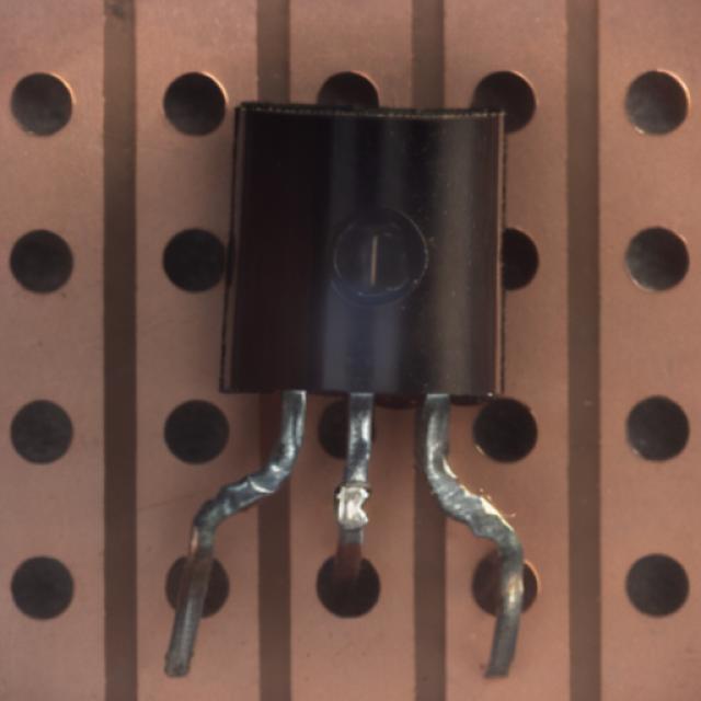
The MVTec Combined Industrial Object Defects dataset is a fully synthetic object detection set built around 4 part families that recur across electronics and mechanical assembly: cables, transistors, metal nuts, and screws. It contains 1,000 images across 20 annotation classes, with YOLO-format bounding box annotations.
| Coverage axis | Value |
|---|---|
| Total images | 1,000 |
| Part families | 4 |
| Annotation classes | 20 |
| Resolution | Mixed |
| Annotation format | YOLO bounding boxes |
| Real-world footage used | 0% |
The twenty classes are deliberately granular. Rather than a single "cable defect" label, the cable family alone breaks into distinct failure modes: bent wire, cable swap, cut inner insulation, cut outer insulation, missing cable, missing wire, and poke insulation. The transistor, metal nut, and screw families decompose the same way, into specific physical and assembly faults rather than a generic anomaly flag.
That granularity matters for a practical reason. A model trained to flag "something is wrong" tells an operator nothing actionable. A model that distinguishes a cut outer insulation from a missing wire maps directly onto different root causes and different line interventions. Class-level specificity is what makes a detector useful on a real factory floor rather than just on a dashboard.
Every image in the dataset is 100% synthetically generated, with no real-world footage used. The annotations are bounding boxes in normalized YOLO format, and the catalog records the resolution as Mixed, reflecting the different capture geometries each component type implies.
Reading the Class Distribution
The most instructive part of this dataset is not the images. It is the class balance, because it makes the coverage problem visible.
Most classes sit at exactly 50 images, which is the floor the dataset was engineered to guarantee. A few classes carry more, driven by how many defect instances appear per image. cable_missing_wire reaches 87 total objects across 50 images, averaging 1.74 instances per image, while transistor_cut_lead reaches 86 objects at 1.72 per image. Other classes, like transistor_misplaced or metal_nut_flip, are strictly 1 instance per image.
This is exactly the kind of even floor that real-world capture almost never produces. In a dataset scraped from production, the per-class counts would be wildly skewed toward whatever the line happens to fail at most often, and the rare classes would be represented by a handful of examples or none. Here, every defect type clears a deliberate minimum. That is coverage engineering rather than coverage luck.
The object-area statistics tell a second story that any detection engineer will recognize. The classes do not just differ in frequency. They differ in scale by nearly two orders of magnitude. A metal nut flip occupies on average 76.22% of the frame, and a transistor misplaced occupies 59.71%, while a transistor cut lead occupies just 0.69% and a screw manipulated front occupies 1.68%.
| Class statistic | Example class | Value |
|---|---|---|
| Highest object count | cable_missing_wire |
87 objects |
| Highest instance density | cable_missing_wire |
1.74 objects/image |
| Highest object count, transistor family | transistor_cut_lead |
86 objects |
| Highest instance density, transistor family | transistor_cut_lead |
1.72 objects/image |
| Large average object area | metal_nut_flip |
76.22% of frame |
| Large average object area | transistor_misplaced |
59.71% of frame |
| Small average object area | transistor_cut_lead |
0.69% of frame |
| Small average object area | screw_manipulated_front |
1.68% of frame |
A detector has to handle a defect that fills the frame and a defect that is a fraction of a percent of it, in the same model, across the same classes. Small-object detection is a well-known weak point for standard architectures, and a dataset that mixes frame-filling and near-invisible defects forces that weakness into the open rather than hiding it behind a forgiving average object size.
Spatial and Co-occurrence Structure
Two further properties of the dataset are worth attention because they speak to evaluation integrity, not just training volume.
The dataset publishes per-class spatial heatmaps showing where each defect type tends to fall in the frame. This is the kind of diagnostic that catches positional bias before it poisons a model. If every example of a class sits in the same corner, a detector can learn the corner instead of the defect, and the resulting model collapses the moment a real part is framed differently. Surfacing spatial density per class is how you catch that failure mode at the data stage rather than in production.
The co-occurrence structure is intentionally clean. Each class appears as a standalone defect rather than tangled with others in the same frame. For a dataset whose job is to teach a detector what each specific failure mode looks like, isolating one defect type per image is a defensible design choice: it keeps the learning signal for each class uncorrelated from the others, so the model is not quietly learning that two defects always travel together when they do not.
These are not glamorous features. They are the difference between a dataset that produces a number and a dataset that produces a model you can defend in front of a domain expert.
What the Model Actually Achieved
A dataset's claims are only as good as the validation behind them. Here the result is stated with the experimental setup attached, which is the only way a benchmark is worth reporting.
A YOLOv8 detector, reference checkpoint yolov8m.pt, was trained on the synthetic images and evaluated on a held-out set. The reported validation metrics are 0.8996 mAP@0.5, 0.6852 mAP@0.5:0.95, 0.8771 Precision, and 0.8490 Recall.
| Metric | Reported value |
|---|---|
| Training data | 100% synthetic images |
| Validation data | 100% real held-out images |
| Model checkpoint | yolov8m.pt |
mAP@0.5 |
0.8996 |
mAP@0.5:0.95 |
0.6852 |
Precision |
0.8771 |
Recall |
0.8490 |
The setup is the part that matters. These results come from training on 100% synthetic images and validating on 100% real-world held-out images. That is the hard version of the test. A model trained on synthetic data and validated on synthetic data tells you almost nothing, because it can exploit rendering artifacts that will never appear in production. Training on synthetic and validating on real is the configuration that actually measures whether the synthetic distribution transferred to reality.
Reaching roughly 0.90 mAP@0.5 under that constraint is a meaningful signal that the synthetic coverage maps onto real defects rather than onto a synthetic look. The stricter mAP@0.5:0.95 figure of 0.6852 is the honest counterweight: localization tightens up less than detection does, which is consistent with the small-object and scale-variance challenges the class statistics predicted.
One caveat belongs in plain sight. These figures describe this dataset's held-out real validation set, not any particular factory's parts. The dataset documentation itself recommends mixing real images into the training set for production use rather than relying on synthetic data alone. For production deployments, AnywayLabs recommends mixing 10-25% real images into the training set. Synthetic data builds the coverage floor. A modest amount of real data closes the domain gap for a specific deployment. Treating synthetic as a complete replacement for real capture overstates what any synthetic set, including this one, can do on its own.
| Deployment role | Recommended share |
|---|---|
| Synthetic data | 75-90% |
| Real target-environment images | 10-25% |
Where Synthetic Coverage Fits
The argument for synthetic data in industrial inspection is narrower and more durable than the marketing version. It is not that synthetic images replace real ones. It is that synthetic generation is the only practical way to make rare defect coverage even.
You cannot wait for a production line to fail in 20 distinct ways enough times to build a balanced dataset. By the time you have collected enough real examples of the rarest assembly errors, the cost of the misses you tolerated while collecting them has already exceeded the cost of the inspection system. Synthetic generation inverts that: the rare classes get the same coverage floor as the common ones, on day 1, under controlled and varied conditions.
That is what the class distribution in this dataset demonstrates. Every defect type clears a deliberate minimum, object scales span the full range a detector must handle, and spatial placement is diagnosed rather than assumed. The 0.90 mAP@0.5 result, earned against real validation images, is downstream of that coverage discipline rather than separate from it.
The dataset is open, YOLO-formatted, and available on both Hugging Face and the AnywayLabs catalog. It is a useful starting point for anyone building automated visual inspection who has felt the gap between a strong aggregate score and a model that misses the defect that mattered.
The MVTec Combined Industrial Object Defects dataset is available on Hugging Face and the AnywayLabs dataset catalog.